The analysis operations in these tutorials are as follows:
1)Connectivity distribution. Display a graph showing how many pores have ink-bottle pores (pores with only one throat connected).
2)Content distribution. Determine the content distribution in the z-direction
a)For a wetting fluid (Water intruding into the top of the unit cell for 500 ms, with 10 intermediate structures)
i)Compare the fluid uptake for a wetting simulation over the same time period with a small applied pressure i.e 0.001 MPa. (Repeat the above operation with the applied pressure.)
b)For a non-wetting fluid (Not used in the tutorial system but works in exactly the same way and can use the same instructions)
The following two tutorials are not yet included in the pdf and print versions of the manual.
3)Microtoming. Generate a histogram for granite sample and export the histogram data as a spreadsheet file.
4)Fluid uptake progress.
a)Conversion of wetting simulation data to graphical analysis of wetting versus time to check wetting versus square root of time.
i)Compare the fluid uptake for a wetting simulation over the same time period with a small applied pressure i.e 0.001 MPa.
b)Non-wetting fluid uptake graph created of pressure versus intrusion.
Starting off - initialisation of a different type of sample
To provide some contrast to Initialisation tutorials, this tutorial uses a mercury intrusion curve for granite, which has very low porosity (2%), located in your directory: ...\Documents\PoreXpert\Example Files\Experimental Data\Porosimetry .
As revision of the Initialisation tutorial, load the granite.csv file, and try to fit it with a 15x15x15 unit cell, using structure types Vertically banded, Horizontal: Large surface throats, and Horizontal: Large to small. (You can try the other structure types if you wish, as described below, although the small centre zone and large centre zone structures take a long time to fit. )
The example results in this set of tutorials are based on our own fits, contained in the granite learn 15x 3fits.pXt file accessible from the downloads page of the website. These are likely to be better than yours, because our software has learned from experience. You can switch your own learning mode off if you wish, as shown below, but it is not advised.
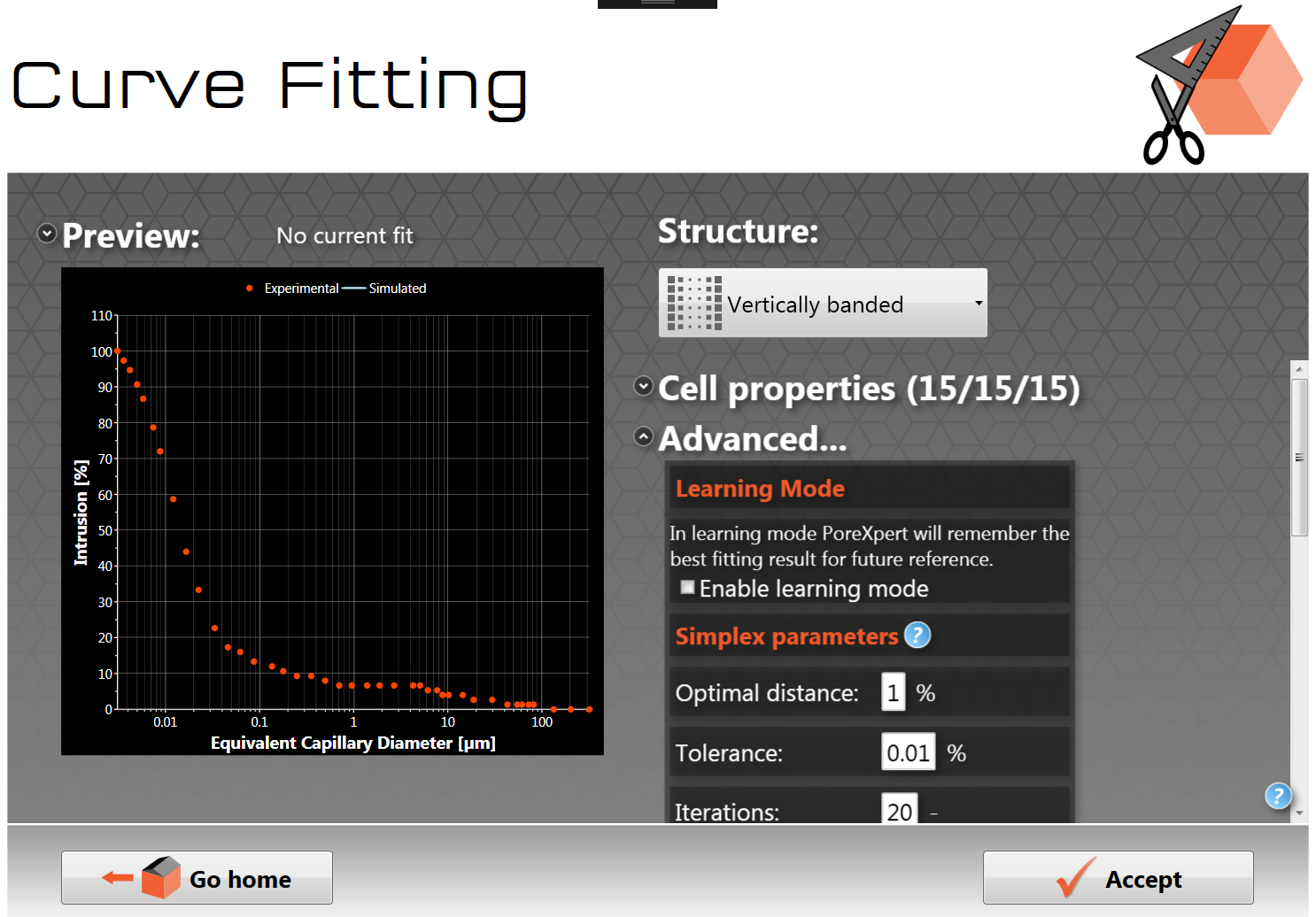
Curve fitting screen with Enable learning mode unclicked - which is not recommended.
Alternative sample files
Clashac outcrop sandstone
To use the straightforward fit from the Initialisation tutorial, load the file Clashac initialisation results.pXt . The example results in this set of analysis operations tutorials are calculated with this file.
Fertiliser
The fertiliser data file (Fertiliser.csv) is a more complicated data file than the data files previously used in the tutorial. it is recommended when fitting the data file that the number of iterations is increased from 20 to 50 iterations per temperature. The number of iterations can be changed in the advanced options on the simplex page.
The additional data file Fertiliser different fits.pxt, contains three simplex fits of the experimental data: the first fit shows the unit cell using the default fitting parameters, the second structure shows the unit cell after increasing the number of iterations and the third fit shows a large cubic unit cell 25 x 25 x 25.