Having established that the optimum structure type for our medicinal tablet is Horizontal: Large to small, then we now need to establish which stochastic realisation is best. We refer to each stochastic realisation by its stochastic generation number. The random (Monte Carlo) nature of inverse modelling involves the use of random numbers. However, a true random number generator will produce different random numbers, and hence different answers, every time that the model is run, whereupon it is impossible to know whether the differences are due merely to the stochastic realisation process, or some other factor. That uncertainty is eliminated by using a pseudo-random number generator (a Mersenne Twister) which is re-seeded with the same first seed for every session. That means that, if the learning mode is switched off as at present, your results should be the same as in this example.
So - File | Open to open a new datafile, and reload the Medicinal tablet edited.csv file, and Accept. Then Go home, PoreBatch, Open batch description, open the file Medicinal_Tablet_fitting_5_stoch_gens_HLtoS_noLearn.pXt , and PoreBatch | Run batch list.
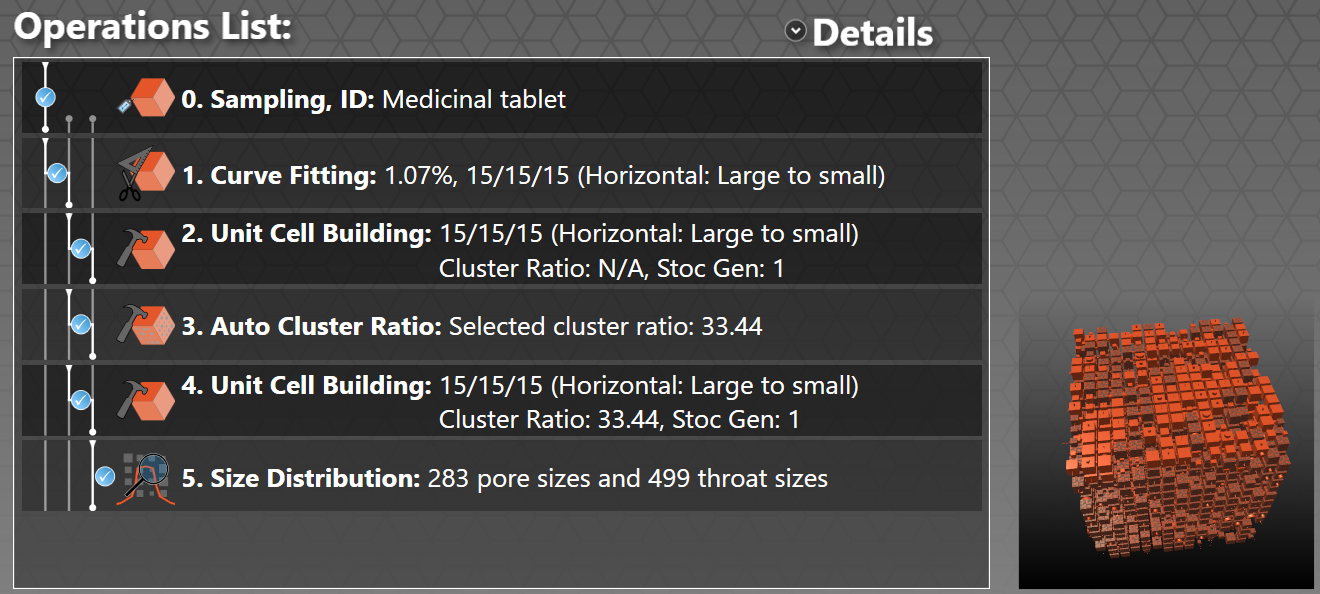
Once the batch has completed, your Operations List should look like this:
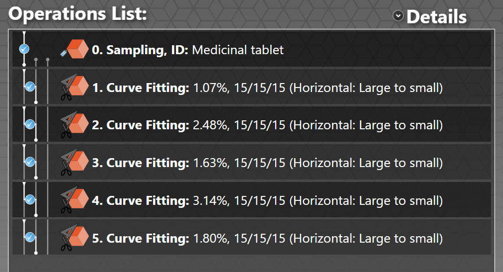
The batch file was written so for this run the operation number on the left corresponds to the stochastic generation number. However, that is not necessarily the case with your own fits. To check on the quality of fit represented by a particular Curve Fitting operation, simply double click on it. The fit is then shown in a graph on the left, and the stochastic generation number is listed in the Parameters... drop-down menu.
It would be tempting at this point to assume that the best choice in this case is stochastic generation 1, because that has the optimum fit (1.07 %). For some samples that are difficult to fit, for example Gilsocarbon graphite or tight oil shale that have their size ranges extended to small sizes using surface are and pycnometry measurements, then the closest distance is usually the one to choose, because other stochastic generations give rise to much worse fits. Sometimes proves even more difficult to obtain structures. In that case attempt to model several of the samples. If one produces a fit, then note the simplex fitting parameter values. Then for the other samples, which have proved impossible to fit, on the Curve Fitting screen go to the Advanced... dropdown menu, and in the Simplex limits section constrain the simplex to values around those that have been successful for the sample that you did manage to fit. (At the very end of this tutorial we will also encounter another over-riding reason to change the selection of stochastic generations.)
However when, as in this case, the curve is relatively straightforward to fit, and there is more than one fit below a distance of 2%, then a tighter method of choosing the stochastic generation can be employed. As well considering fits with distances less than 2%, we also survey the stochastic generations to discover the most statistically central stochastic generation, which may or may not be that with the lowest distance. In this case we generated five stochastic generations to choose from, but that is really the minimum - ten would be safer. Then we know that the PoreXpert model for this sample is representative - i.e. its fitting parameters do not include any outliers. This is especially important when looking at the trends across a series of samples, which is the normal way of using PoreXpert.
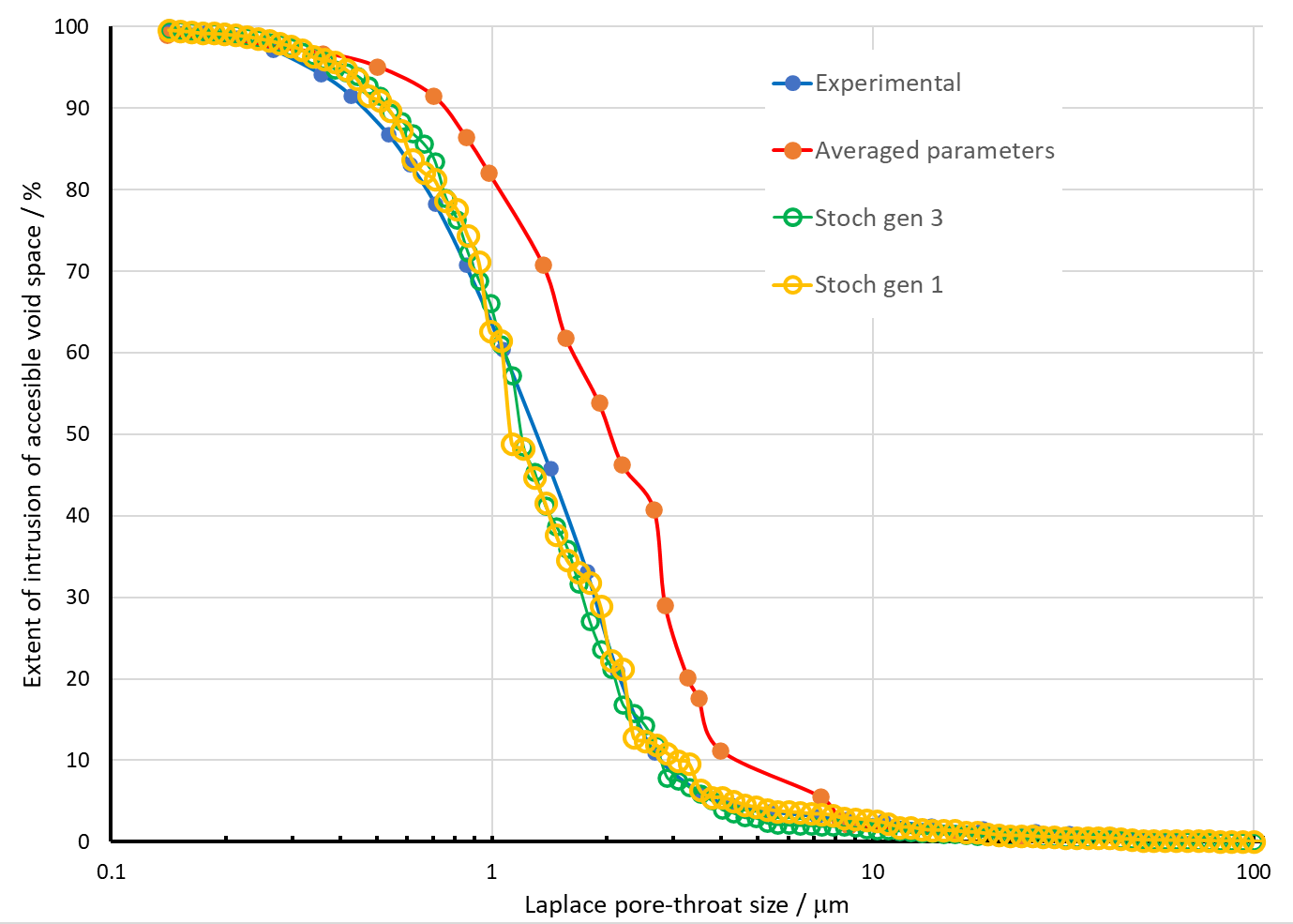
Another temptation is to generate a PoreXpert structure based on the average of each parameter, using the Cell Engineering option. However, that produces a structure with the wrong percolation characteristics as shown below. (The structure shown is averaged in linear, rather than the precise semi-logarithmic parameter space explained below.) The reason is that all the fitting parameters are coupled, not independent - if a particular fit has a high value of one parameter, then other parameters may go low to compensate so that there is still convergence onto the experimental percolation characteristics.
At this point, save the output as a PoreXpert file (File | Save as ... | PoreXpert file ), as we will have to back track as explained below.
To find the representative sample, from the Home, Operations List screen, File | Save as ... | CSV file . Save to a suitable directory on your computer. Go that directory and you should see a file list as shown:
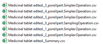
The numbers are the operation numbers, that for this run correspond to the stochastic generation numbers. We need to important specific information from these files into a spreadsheet software - in the present example, we will use MS Excel. The information we need from each sheet are the stochastic generation number (row 10), and Simplex results shown in rows 20 to 25. Import these data for each stochastic generation into a single summary spreadsheet which should look like this:
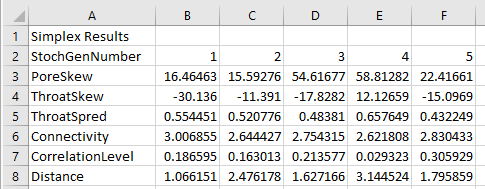
Now calculate the mean and standard deviation (σ) row by row for rows 3 to 7. (To be more precise, the Pore Skew and Throat Skew vary within logarithmic parameter space, so the mean, standard deviations and permitted ranges for these two variables should be in logarithmic parameter space - equivalent to using a geometric rather than arithmetic mean. For simplicity, we have ignored this factor for this exercise.)
Insert a blank row before Distance. The stochastic generation to choose is then the one that has most parameters within the mean ± σ , while also having an acceptable Distance - i.e. less than 2%. Results are Conditionally Formatted according to these criteria in the table below - red is too high, blue too low.
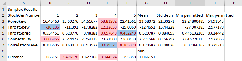
It is clear from this table that the stochastic generation to choose is 3, not 1. Stochastic generation 1 has two outlying parameters - Throat Skew and Connectivity. Stochastic generation 3 has a higher distance, but as can be seen from the graph above, the increase in distance is not significant - it would quite likely be within the experimental scatter if another mercury intrusion curve was measured.
So you can now return to the PoreXpert Operations List screen and delete stochastic generation numbers 1,2, 4 and 5. (Click on each one in turn to highlight it, and press your Delete key). Then you are left with just the correctly chosen stochastic generation of a datafile with minimised artefacts. So File | Save as ... | PoreXpert file to save the file for later.
Your next operation would be to build the unit cell (Run new operation... | Initialisation... | Building ), Accept, then run the Auto Cluster Ratio (Run new operation... | Initialisation... | Auto Cluster ratio ). In this case, the Auto Cluster does not work - manual cluster ratio builds show that there is a major kink in the Unresolved Clusters distribution which the Cluster Ratio cannot eliminate. This is a pertinent demonstration that the stochastic nature of PoreXpert makes it something of an untameable and unpredictable beast. So in this case that might be a reason to revert to stochastic generation 1, for which the Auto Cluster operation does work, as shown below.
However, for real research, you would have the learning mode switched on, and be generating unit cells on a 25x25x25 grid, or 30x30x30 on a supercomputer, for which the Auto Cluster operation is more stable.