At the end of the last tutorial correcting for the blank the home screen showed the raw experimental data and the experimental data corrected for the blank data file. The next step is to determine the appropriate point at which to correct for compression of the sample.
The determination of the appropriate point for the compression correction involves inspecting the graph. As before, to zoom in on the graph use the right mouse button and draw a box around the highest pressure region of the graph on the right hand side, as for example shown below. If you select the wrong part of the graph there is a zoom out button above the graph on the right hand side.
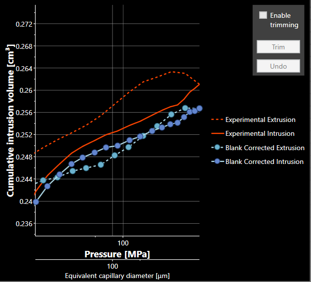
In the case of the tutorial sample, shown above, the first thing to notice is that for the Blank Corrected curves there is no longer an impossible increase of intrusion as the pressure is decreased to form the dashed Experimental Extrusion graph.
You need to choose a point above which you feel the intrusion and extrusion curves lie on top of each other - i.e above which what seems like intrusion is actually just the compression of the sample. In the tutorial example above, this is not very clear - you may well have a clearer example yourself. However, in the example above, we can be fairly sure that the top four points of the intrusion curve (darker blue) are compression, because overall the intrusion and extrusion curves are similar over quite a wide range of the pressure shown in the graph. So we choose 4 as the number of points for the compression correction. In this case, you should find that the bulk modulus and compressibility do not change significantly if a different number of points in the overlapping range is chosen.
You can now go onto the next stage, performing the compression correction.