On the main screen as shown below click Input sample datafile | Open...

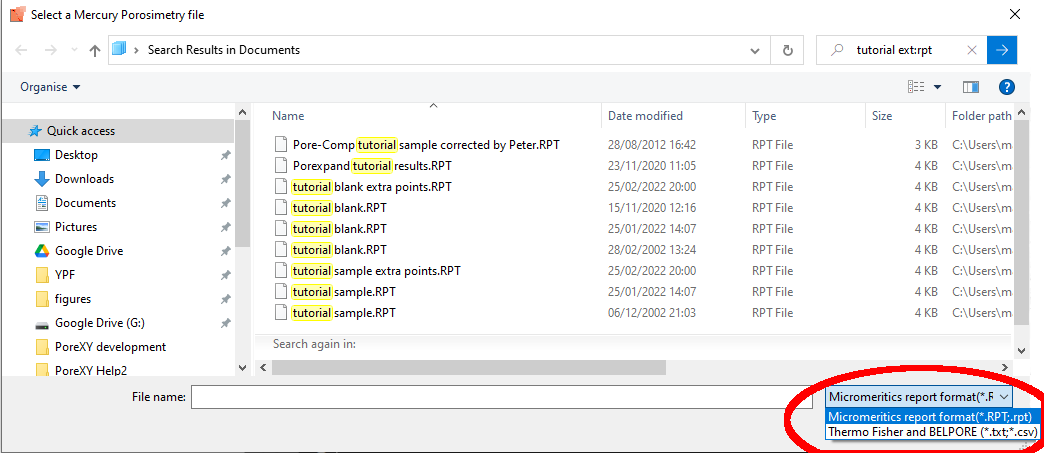
When browsing for a sample file, ensure that the file name filter is set to the correct type using the dropdown menu control as highlighted below. To try out PoreXY, load the file tutorial sample.RPT supplied with the software.
Once the datafile is loaded, unavailable options will disappear from the screen. On these Help pages, we show all operations for the Micromeritics example file (tutorial sample.RPT), as that is the one that has all available operations available to it. We also give occasional examples of outputs from the other example files.
The Micromeritics tutorial sample.RPT datafile requires extra information, and a blank correction, as now explained. After loading this file, the preview screen should now display the following graph:

You can now drag-draw a square with the mouse around the top section of the graph while holding down its right-hand button. This will enlarge that section of the curve that has been targeted, for example as shown:
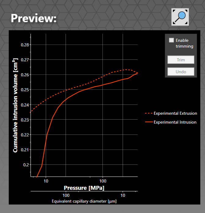
This shows that as the applied pressure is decreased to measure the extrusion curve, shown dashed, the cumulative intrusion volume of mercury increases. That is a physical impossibility that is corrected by the bank correction as described in the following sections. To show the whole graph again, click on the zoom out magnifying glass icon shown at the top of the screenshot above.
For Micromeritics files, additional information has to be input, as shown below. If you are loading a Thermo Fisher or BELPORE file, then the datafiles already contain the extra information and you will already have been required to carry out a blank correction. There are then two alternatives according to whether (i) the compression correction has already been carried out, or (ii) the uncorrected data is being read in. Respectively jump to (i) Determining the start of the compression phase, or (ii) Trimming the graph. If your datafile does not need trimming, then skip to Thinning and exporting data.
For the Micromeritics files, click on the Sample dropdown menu, and check whether all the required information has been provided. The dropdown display shows the properties of the mercury read from the data file and basic information on the sample. In the case of the tutorial sample.RPT file, there is some additional experimental information required for the calculations, which cannot be read from the experimental data files. The following figure shows an expanded view of the sample information, visible if you scroll down.

Expanded sample information on home screen
The information required to perform a complete compression correction is (i) the penetrometer and assembly weight, which is calculated once the penetrometer has been sealed with the sample by subtracting the sample weight from the total assembly and sample weight, and (ii) the weight of the penetrometer with sample filled with mercury at the end of the low pressure stage of the experiment, to allow the software to calculate the volume of the sample, by comparing the filled penetrometer weight with the blank filled penetrometer weight.
Enter the following details into the text boxes shown above, namely:
Penetrometer + assembly weight: 65.3229 g
Penetrometer + assembly + sample + mercury weight: 130.7231 g
You can now continue onto the next stage, performing the blank correction.